
作者:非妃是公主
专栏:《计算机视觉》
个性签:顺境不惰,逆境不馁,以心制境,万事可成。——曾国藩
专栏系列文章
Cannot find reference ‘imread‘ in ‘init.py‘
error: (-209:Sizes of input arguments do not match) The operation is neither ‘array op array‘ (where

图像分类任务
图像可以理解为一个矩阵,如果是彩色图像,就可以理解为一个3层的矩阵,比如3×64×64的RGB图像。每个像素点的值为0~255,图像分类的任务就是通过这个图像矩阵作为输入,输出它所属不同类别的标签。
图像分类所面临的挑战
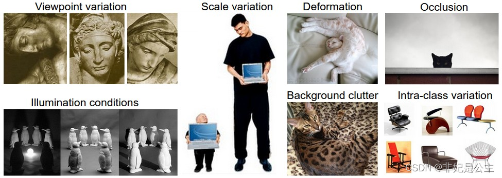
因此,根据以上图像分类任务的要求不难发现,图像分类具有很多挑战:
① 从不同的角度来看,一个物体是不同的。
② 不同的缩放比例,一个物体的大小也是不同的。
③ 不同的形状,一个物体可能有不同的形状,比如躺着的小猫和站着的小猫。
④ 分类目标可能是被遮挡的。
⑤ 光照对物体像素的影响是十分严重的。同一个物体不同光照下,像素差异很大。
⑥ 背景掩护,待分类的对象可能和其背景非常相似,使得他们很难被识别出来。
⑦ 许多物体存在较大的类内差异,比如都是椅子,但不同的椅子外形看起来差别很大。
应对策略
对于以上挑战,采用传统意义上的算法是很难进行准确的分类的,我们无法将这个物体到底属于哪一类用代码描绘出来,所以需要采用数据驱动的方式(Data-driven approach)——它就像我们教小孩子一样,不是直接告诉它,什么是小猫、小狗、杯子……而是给它展示,这就是小猫、小狗、杯子,相同的道理,我们通过某种学习算法来学习这些样例,学习到每种类别的图像到底是什么样子的,这就是数据驱动的方法。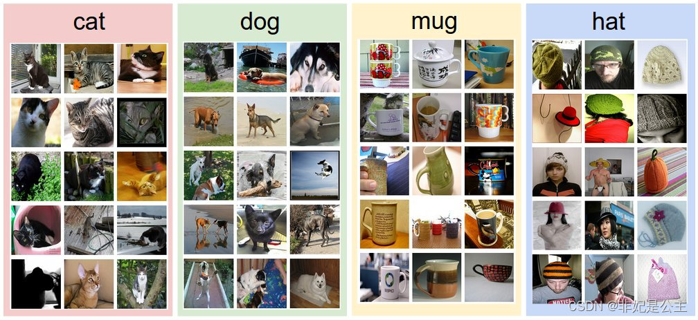
四个视觉类别的训练集例子。实际情况中,可能会有数千的类别和数以千万计的图像样本。
图像分类步骤
学习算法主要分为以下几个步骤:
① 输入(Input):学习算法的输入是一个N张图片的集合,其中,每张图片都标有K个不同类别中的一个,称为标签。我们把这N张图片的集合和标签的整体称为训练集。
② 学习(Learning):通过训练集让学习算法学到每一个类别到底是什么样子的。这也被叫做训练(training)或者学习(learning)
③ 评估(Evalution):最后,通过一个在训练过程中没有用到的图像数据集(测试集),来预测(predict)它们的标签,将预测的结果与测试集的真实标签(ground truth)比对评估模型的学习效果。
最近邻分类
数据集
我们使用CIFAR-10 dataset,这个数据集包含了60000张3×32×32的图像,每个图像被分成了10类(飞机、汽车、鸟等)。这60000张图像被分为50000张的训练集和10000张测试集。
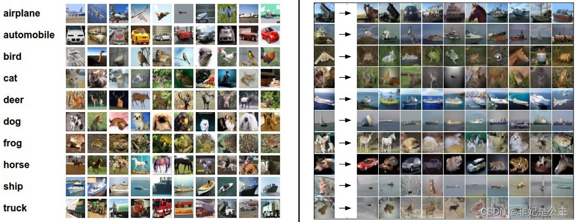
左图:CIFAR-10数据集中的一些样例. 右图:第一列展示了测试集中10个类别的图像,后面的展示了训练集中与这10个图像最相近的图像。
L1距离
从图中可以看出,10张测试图像中只有3张图片是分类正确的,即:最相近的图片和测试图像相同,其它7张图片是分类错误的(随机分类的正确率在10%)。例如第8个样例,训练集中最相近的图像的标签是车,但实际上测试图像是一个马的头部。因为两张图片都具有相同的黑色背景,这使得两张图片的相似度较大。
两张图片的差异就是通过对应像素点之间的差值来衡量的——L1距离(L1 distance):
d
1
(
I
1
,
I
2
)
=
∑
p
∣
I
1
p
−
I
2
p
∣
\boldsymbol{d_1(I_1,I_2)=\sum\limits_p|I_1^p-I_2^p|}
d1(I1,I2)=p∑∣I1p−I2p∣
其中
I
1
,
I
2
\boldsymbol{I_1,I_2}
I1,I2表示两张图像对应像素点展开的向量,p表示像素点的数量。计算过程如下图:
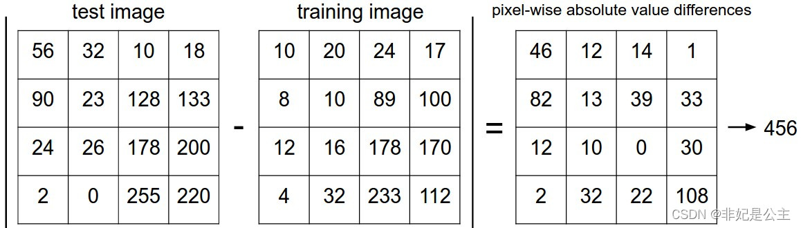
展开向量:
Xtr, Ytr, Xte, Yte = load_CIFAR10('data/cifar10/') # a magic function we provide
# flatten out all images to be one-dimensional
Xtr_rows = Xtr.reshape(Xtr.shape[0], 32 * 32 * 3) # Xtr_rows becomes 50000 x 3072
Xte_rows = Xte.reshape(Xte.shape[0], 32 * 32 * 3) # Xte_rows becomes 10000 x 3072
通过以上代码,我们将图像矩阵转化为了3072维度的向量。
通过下面代码可以训练并评估一个分类器
nn = NearestNeighbor() # create a Nearest Neighbor classifier class
nn.train(Xtr_rows, Ytr) # train the classifier on the training images and labels
Yte_predict = nn.predict(Xte_rows) # predict labels on the test images
# and now print the classification accuracy, which is the average number
# of examples that are correctly predicted (i.e. label matches)
print 'accuracy: %f' % ( np.mean(Yte_predict == Yte) )
下面为分类器内部代码的实现,其中
import numpy as np

class NearestNeighbor(object):
  def __init__(self):
    pass

  def train(self, X, y):
    """ X is N x D where each row is an example. Y is 1-dimension of size N """
    # the nearest neighbor classifier simply remembers all the training data
    self.Xtr = X
    self.ytr = y

  def predict(self, X):
    """ X is N x D where each row is an example we wish to predict label for """
    num_test = X.shape[0]
    # lets make sure that the output type matches the input type
    Ypred = np.zeros(num_test, dtype = self.ytr.dtype)

    # loop over all test rows
    for i in range(num_test):
      # find the nearest training image to the i'th test image
      # using the L1 distance (sum of absolute value differences)
      distances = np.sum(np.abs(self.Xtr - X[i,:]), axis = 1)
      min_index = np.argmin(distances) # get the index with smallest distance
      Ypred[i] = self.ytr[min_index] # predict the label of the nearest example

    return Ypred
通过下面代码计算L1距离
distances = np.sum(np.abs(self.Xtr - X[i,:]), axis = 1)
其中对,得到的距离进行可视化如下灰度图,越亮的位置代表L1值越大,距离越大:
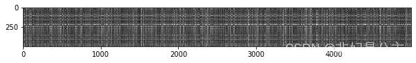
其中每一行代表一个测试样例(0~500)到它的训练样本的距离(0~5000)。
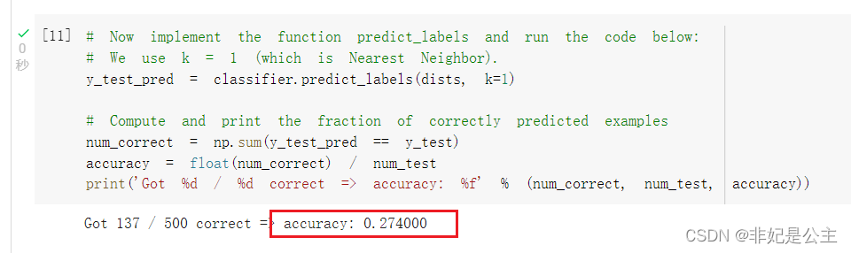
实现NearestNeighbor类后,在colab上运行上面代码,可以看到分类器的分类正确率在27%左右。
L2距离
有不同的距离来计算两个向量直接按的距离,另一个比较常用的选择就是L2距离(L2 distance)
d
2
(
I
1
,
I
2
)
=
∑
p
(
I
1
p
−
I
2
p
)
2
\boldsymbol{d_2(I_1,I_2)=\sqrt{\sum\limits_p(I_1^p-I_2^p)^2}}
d2(I1,I2)=p∑(I1p−I2p)2
这次,对两个向量的差先平方,再求和,最后开放,不再同L1距离一样直接将两个向量的差取绝对值然后求和。
distances = np.sqrt(np.sum(np.square(self.Xtr - X[i,:]), axis = 1))
L1 vs. L2
由于L2距离存在一个平方的过程,这会使得许多中等大小的数变成一个非常大的数,因此,两个向量之间的差距被放大。
K-近邻分类
根据K-近邻算法,以及上述定义的损失函数,可以得到如下结果,关于K-近邻算法的具体说明可以参考机器学习08:最近邻学习,最终得到的分类结果,如下:
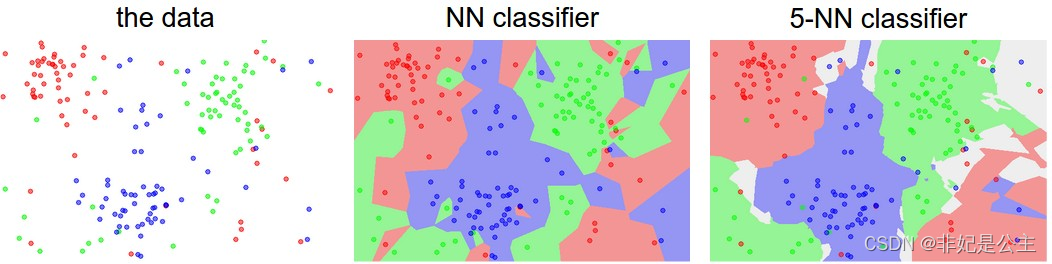
从图中不难发现,最近邻(1-近邻)算法的边角十分分明,也就是说,会存在过拟合的情况,而5-近邻过拟合的情况得到了一定的缓解!其中空白区域部分的面积为2:2:1的情况,这种情况下,由于存在两个最大可能的类别,因此分类器无法判定到底属于哪一类,所以不去进行分类。
矩阵运算与循环运算效率比较
值得注意的是,在进行矩阵运算的时候,由于可以利用GPU的并行运算的特性,采用矩阵运算可以大大加快模型的求运行速度,对于KNN算法,采用矩阵运算、一层循环、两层循环对算法分别进行实现后,如下:
# Let's compare how fast the implementations are
def time_function(f, *args):
    """
    Call a function f with args and return the time (in seconds) that it took to execute.
    """
    import time
    tic = time.time()
    f(*args)
    toc = time.time()
    return toc - tic

two_loop_time = time_function(classifier.compute_distances_two_loops, X_test)
print('Two loop version took %f seconds' % two_loop_time)

one_loop_time = time_function(classifier.compute_distances_one_loop, X_test)
print('One loop version took %f seconds' % one_loop_time)

no_loop_time = time_function(classifier.compute_distances_no_loops, X_test)
print('No loop version took %f seconds' % no_loop_time)

# You should see significantly faster performance with the fully vectorized implementation!

# NOTE: depending on what machine you're using,
# you might not see a speedup when you go from two loops to one loop,
# and might even see a slow-down.
效果如下:
Two loop version took 38.739486 seconds
One loop version took 23.500014 seconds
No loop version took 0.336616 seconds
可以很明显的看出,矩阵运算效率远高于循环运算!因此,后续在处理图像的时候我们应该多使用矩阵运算以利用GPU的并行能力。
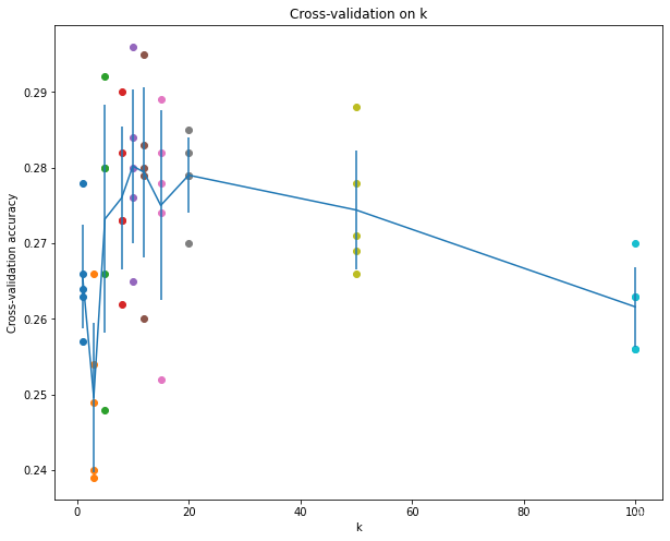
超参数的选择
由于K近邻算法中的K值属于一个超参数,因此需要进行选择。而选择合适的超参数是采用实验的方法,在测试集上运行模型,观测哪一个超参数下模型的准确率最高,代码如下:
num_folds = 5
k_choices = [1, 3, 5, 8, 10, 12, 15, 20, 50, 100]

X_train_folds = []
y_train_folds = []
################################################################################
# TODO:                                                                        #
# Split up the training data into folds. After splitting, X_train_folds and    #
# y_train_folds should each be lists of length num_folds, where                #
# y_train_folds[i] is the label vector for the points in X_train_folds[i].     #
# Hint: Look up the numpy array_split function.                                #
################################################################################
# *****START OF YOUR CODE (DO NOT DELETE/MODIFY THIS LINE)*****

# split self.X_train to 5 folds
avg_size = int(X_train.shape[0] / num_folds) # will abandon the rest if not divided evenly.
for i in range(num_folds):
    X_train_folds.append(X_train[i * avg_size : (i+1) * avg_size])
    y_train_folds.append(y_train[i * avg_size : (i+1) * avg_size])

# *****END OF YOUR CODE (DO NOT DELETE/MODIFY THIS LINE)*****

# A dictionary holding the accuracies for different values of k that we find
# when running cross-validation. After running cross-validation,
# k_to_accuracies[k] should be a list of length num_folds giving the different
# accuracy values that we found when using that value of k.
k_to_accuracies = {}


################################################################################
# TODO:                                                                        #
# Perform k-fold cross validation to find the best value of k. For each        #
# possible value of k, run the k-nearest-neighbor algorithm num_folds times,   #
# where in each case you use all but one of the folds as training data and the #
# last fold as a validation set. Store the accuracies for all fold and all     #
# values of k in the k_to_accuracies dictionary.                               #
################################################################################
# *****START OF YOUR CODE (DO NOT DELETE/MODIFY THIS LINE)*****

for k in k_choices:
    accuracies = []
    print(k)
    for i in range(num_folds):
        X_train_cv = np.vstack(X_train_folds[0:i] + X_train_folds[i+1:])
        y_train_cv = np.hstack(y_train_folds[0:i] + y_train_folds[i+1:])
        X_valid_cv = X_train_folds[i]
        y_valid_cv = y_train_folds[i]

        classifier.train(X_train_cv, y_train_cv)
        dists = classifier.compute_distances_no_loops(X_valid_cv)
        accuracy = float(np.sum(classifier.predict_labels(dists, k) == y_valid_cv)) / y_valid_cv.shape[0]
        accuracies.append(accuracy)
    k_to_accuracies[k] = accuracies

# *****END OF YOUR CODE (DO NOT DELETE/MODIFY THIS LINE)*****

# Print out the computed accuracies
for k in sorted(k_to_accuracies):
    for accuracy in k_to_accuracies[k]:
        print('k = %d, accuracy = %f' % (k, accuracy))
输出结果如下:
1
3
5
8
10
12
15
20
50
100
k = 1, accuracy = 0.263000
k = 1, accuracy = 0.257000
k = 1, accuracy = 0.264000
k = 1, accuracy = 0.278000
k = 1, accuracy = 0.266000
k = 3, accuracy = 0.239000
k = 3, accuracy = 0.249000
k = 3, accuracy = 0.240000
k = 3, accuracy = 0.266000
k = 3, accuracy = 0.254000
k = 5, accuracy = 0.248000
k = 5, accuracy = 0.266000
k = 5, accuracy = 0.280000
k = 5, accuracy = 0.292000
k = 5, accuracy = 0.280000
k = 8, accuracy = 0.262000
k = 8, accuracy = 0.282000
k = 8, accuracy = 0.273000
k = 8, accuracy = 0.290000
k = 8, accuracy = 0.273000
k = 10, accuracy = 0.265000
k = 10, accuracy = 0.296000
k = 10, accuracy = 0.276000
k = 10, accuracy = 0.284000
k = 10, accuracy = 0.280000
k = 12, accuracy = 0.260000
k = 12, accuracy = 0.295000
k = 12, accuracy = 0.279000
k = 12, accuracy = 0.283000
k = 12, accuracy = 0.280000
k = 15, accuracy = 0.252000
k = 15, accuracy = 0.289000
k = 15, accuracy = 0.278000
k = 15, accuracy = 0.282000
k = 15, accuracy = 0.274000
k = 20, accuracy = 0.270000
k = 20, accuracy = 0.279000
k = 20, accuracy = 0.279000
k = 20, accuracy = 0.282000
k = 20, accuracy = 0.285000
k = 50, accuracy = 0.271000
k = 50, accuracy = 0.288000
k = 50, accuracy = 0.278000
k = 50, accuracy = 0.269000
k = 50, accuracy = 0.266000
k = 100, accuracy = 0.256000
k = 100, accuracy = 0.270000
k = 100, accuracy = 0.263000
k = 100, accuracy = 0.256000
k = 100, accuracy = 0.263000
代码
为了逻辑的连续性,本文省略了一些细节,用到的详细代码已放置到代码仓库,github仓库地址:https://github.com/ManYufei888/cs231n
版权声明:本文内容由互联网用户自发贡献,该文观点仅代表作者本人。本站仅提供信息存储空间服务,不拥有所有权,不承担相关法律责任。如发现本站有涉嫌侵权/违法违规的内容, 请发送邮件至 举报,一经查实,本站将立刻删除。
文章由极客之家整理,本文链接:https://www.bmabk.com/index.php/post/130487.html